HDBSCAN an efficient and flexible clustering technique

2024-01-01 2024-01-01 1196 words 6 minutes

Contents

1 Introduction

Clustering is a unsupervised machine learning method of grouping data points so that points in the same group are more similar to each other than the points in other groups. Clustering is used in fields like pattern recognition, data mining for grouping related data, in market segmentation to identify distinct customer groups based on behavior or preferences and many more.

HDBSCAN is a clustering algorithm which is an extension of another method named DBSCAN. This article assumes understanding of different clustering techniques especially density based and hierarchical based clustering. In this article, I will give a brief overview of DBSCAN and then present it’s improved variant HDBSCAN and highlight their differences.

2 Brief overview of DBSCAN

DBSCAN identifies clusters based on density of the data points and marks low density regions as outliers. DBSCAN does not require the number of clusters to be set in advance which some other methods such as K-Means, K-Medoids do. It requires two parameters epsilon and minPts. Epsilon defines the neighborhood radius and minPts is the minimum number of points(inside the radius) required for a point to be dense.

DBSCAN can discover clusters of arbitrary shapes which distinguishes it from more simplistic, centroid based algorithms. However, its accuracy depends heavily on the choice of the input parameters and it may be ineffective with data of varying densities. Another disadvantage of DBSCAN is that it doesn’t provide any relation between different clusters, which hierarchical clustering methods do.

3 Introduction to HDBSCAN

HDBSCAN was developed to address some of the inherent shortcomings of DBSCAN. It works better for clustering of complex datasets. The only required parameter for HDBSCAN is the minimum cluster size. It builds a hierarchy of clusters. This hierarchical approach not only aids in understanding the data structure at different scales but also in identifying clusters that persist over varying density levels, offering a more nuanced view of the data which was not possible with DBSCAN.

DBSCAN is very sensitive to the parameters epsilon and minPts. A good understanding of the dataset is a pre requisite to fine tune these parameters. On the other hand, HDBSCAN automatically determinse an optimal clustering scale based on the data which significantly reduces the need for parameter tuning. This makes HDBSCAN more user friendly, especially for users who do not have a deep understanding of the underlying structure of their dataset.

4 How HDBSCAN works

The first step is transforming the data space according to density, which is quite similar to DBSCAN. But instead of using a single density threshold (epsilon), it builds a hierarchy of clusters based on varying densities. This hierarchy is created by treating cluster formation as a density contour problem, where contours in data density are identified at different levels, creating a dendrogram.

HDBSCAN uses mutual reachability distance which ensures that points within denser areas are closer together in the transformed space. The hierarchy building step is similar to AGNES. It starts by treating each data point as a separate cluster. Then these points are merged into clusters based on their mutual reachability distance. The height of the merge in the tree indicates the distance at which clusters merged, illustrating the density landscape of the data. Then the tree is condensed by pruning branches that don’t meet the minimum cluster size criterion.

The clusters are extracted from the condensed tree. Unlike DBSCAN, which extracts clusters at a single density level, HDBSCAN extracts clusters persisting over a range of density levels, offering greater flexibility in identifying clusters of varying densities.

5 Finding clusters with varying density

We will generate a dataset of 2d points, one set of them will be dense with a low standard deviation and the other set will be sparse with a higher standard deviation. Then we will run both DBSCAN and HDBSCAN on that dataset.

We can use sklearn library for the creating of such dataset

1
2
3
4
5
6
7
from sklearn.datasets import make_blobs

np.random.seed(42)

dense_blob, _ = make_blobs(n_samples=200, centers=[[0, 0]], cluster_std=0.3)
sparse_blob, _ = make_blobs(n_samples=80, centers=[[3, 3]], cluster_std=0.6)
X = np.vstack([dense_blob, sparse_blob])

Note: Here, a seed is specified for the randomness, so that this result is reproducible

 1
 2
 3
 4
 5
 6
 7
 8
 9
10
11
12
13
14
15
16
17
18
19
20
21
22
23
24
25
26
27
import matplotlib.pyplot as plt
import numpy as np
from sklearn.datasets import make_moons
from sklearn.cluster import DBSCAN
from hdbscan import HDBSCAN

# Apply DBSCAN
dbscan = DBSCAN(eps=0.2)
dbscan_labels = dbscan.fit_predict(X)

# Apply HDBSCAN
hdbscan = HDBSCAN(min_cluster_size=45)
hdbscan_labels = hdbscan.fit_predict(X)

# Plotting
fig, axes = plt.subplots(1, 2, figsize=(12, 5))

# DBSCAN plot
axes[0].scatter(X[:, 0], X[:, 1], c=dbscan_labels, cmap='viridis', s=5)
axes[0].set_title('DBSCAN Clustering')

# HDBSCAN plot
axes[1].scatter(X[:, 0], X[:, 1], c=hdbscan_labels, cmap='viridis', s=5)
axes[1].set_title('HDBSCAN Clustering')

plt.tight_layout()
plt.show()

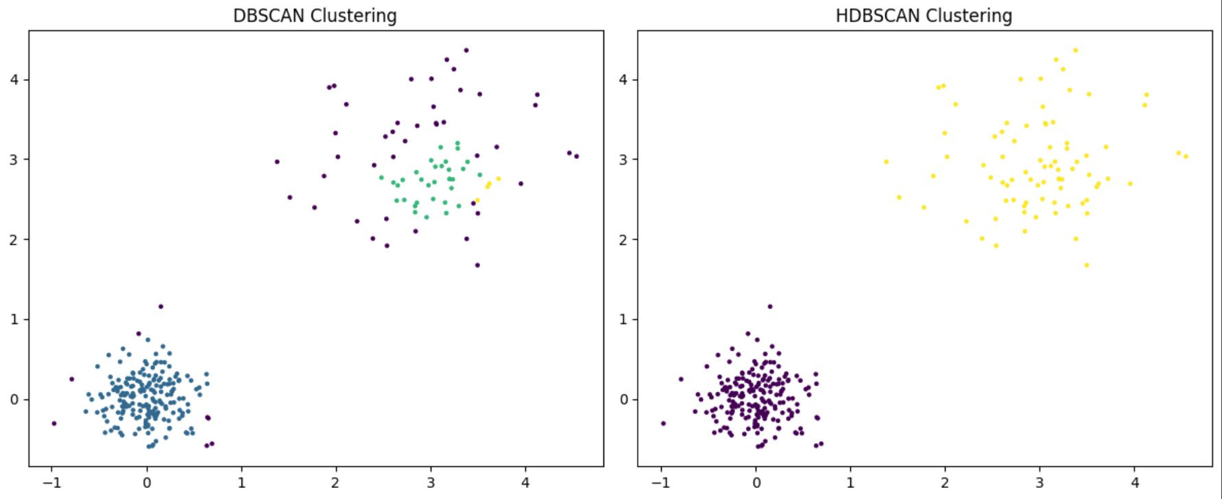
We can see that HDBSCAN recognizes the two clusters while DBSCAN labels most of points on the top left as noise.

6 The hierarchical aspect of HDBSCAN

As we have discussed before HDBSCAN generates a condensed tree which we can plot and analyze. Lets create another dataset of 2d points, but this time we will have two dense cluster and one sparse cluster.

1
2
3
4
5
6
7
np.random.seed(42)
dense_blob1, _ = make_blobs(n_samples=100, centers=[[-5, 0]], cluster_std=0.4)
dense_blob2, _ = make_blobs(n_samples=100, centers=[[0, 5]], cluster_std=0.4)
sparse_blob, _ = make_blobs(n_samples=50, centers=[[3, 3]], cluster_std=1)

# Combine the blobs
X = np.vstack([dense_blob1, dense_blob2, sparse_blob])

As HDBSCAN is a hierarchical clustering method, we can easily plot the dendrogram as well.

 1
 2
 3
 4
 5
 6
 7
 8
 9
10
11
12
13
14
15
16
17
18
19
20
21
22
23
24
25
26
27
28
29
30
31
32
from scipy.cluster.hierarchy import dendrogram

# Perform HDBSCAN
clusterer = hdbscan.HDBSCAN(min_cluster_size=20, gen_min_span_tree=True)
clusterer.fit(X)

# Plotting the clustered data
plt.figure(figsize=(12, 6))
plt.subplot(121)
plt.scatter(X[:, 0], X[:, 1], c=clusterer.labels_, cmap='viridis', s=10)
plt.title("Clustered Data")
plt.xlabel("Feature 1")
plt.ylabel("Feature 2")

# Convert the HDBSCAN single linkage tree to a linkage matrix
linkage_matrix = clusterer.single_linkage_tree_.to_numpy()

# Create the dendrogram
plt.subplot(122)
dendrogram(linkage_matrix)
plt.title('HDBSCAN Dendrogram')
plt.xlabel("Data Point Index")
plt.ylabel("Distance")
plt.tick_params(
    axis='x',
    which='both',
    bottom=False,
    top=False,
    labelbottom=False)

plt.tight_layout()
plt.show()

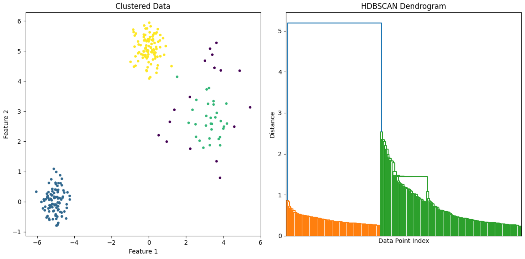
From the dendrogram we can estimate what would be optimal number of clusters for a dataset. It gives us an easy way to visualize the data density and understand the cluster hierarchies.

1
2
3
4
5
6
7
import seaborn as sns

# Access the condensed tree
tree = clusterer.condensed_tree_

# Plot the condensed tree
tree.plot(select_clusters=True, selection_palette=sns.color_palette())

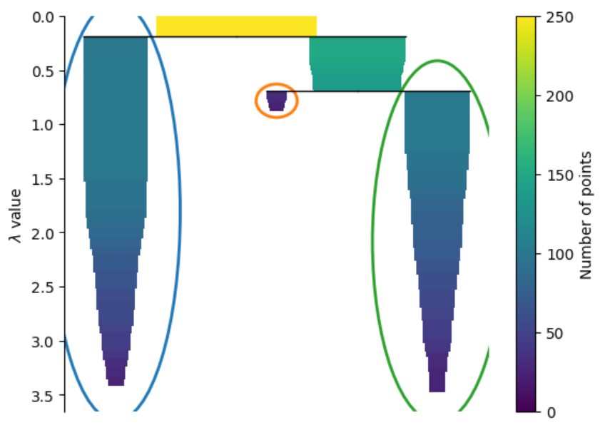
We can visualize the hierarchical relationship between clusters from the condensed tree. You can see which clusters are formed first at the lower levels of density and as the threshold for density decreases these clusters merge together.

7 Summary

HDBSCAN retains the advantages of density based clustering but mitigates some of its limitations. It introduces several key improvements that address the shortcomings of DBSCAN. Their differences are summarized as follows.

HDBSCAN outputs better clustering than DBSCAN when there are varying density within the dataset.
DBSCAN is sensitive to changes in its parameter, epsilon and minPts. HDBSCAN doesn’t require any of these parameters to be set.
HDBSCAN only requires minimum cluster size as a parameter which is much easier to set than epsilon and minPts.
HDBSCAN’s hierarchical method provides a nuanced cluster analysis, as opposed to DBSCAN’s flat clustering approach.